XGBoost

info

Refer: Official doc

Objective function

A salient characteristic of objective functions is that they consist two parts: training loss and regularization term:

$$\operatorname{obj}(\theta)=L(\theta)+\Omega(\theta)$$

where L is the training loss function, and Ω is the regularization term. The training loss measures how predictive our model is with respect to the training data. A common choice of L is the mean squared error, which is given by

$$L(\theta)=\sum_{i}\left(y_{i}-\hat{y}_{i}\right)^{2}$$

Another commonly used loss function is logistic loss (log-likelihood), to be used for logistic regression:

$$L(\theta)=\sum_{i}\left[y_{i} \ln \left(1+e^{-\hat{y}_{i}}\right)+\left(1-y_{i}\right) \ln \left(1+e^{\hat{y}_{i}}\right)\right]$$

The regularization term is what people usually forget to add. The regularization term controls the complexity of the model, which helps us to avoid overfitting.

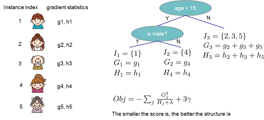
Tree Model with num_iteration K :where K is the number of trees, f is a function in the functional space

$$\hat{y}_{i}=\sum_{k=1}^{K} f_{k}\left(x_{i}\right), f_{k} \in \mathcal{F}$$

Extreme boosting

• https://xgboost.readthedocs.io/en/stable/tutorials/model.html#tree-boosting

For $t \in [0,K]$ , pluggin the above expressions,

$$\begin{aligned} \mathrm{obj}^{(t)} &=\sum_{i=1}^{n} l\left(y_{i}, \hat{y}_{i}^{(t)}\right)+\sum_{i=1}^{t} \Omega\left(f_{i}\right) \\ &=\sum_{i=1}^{n} l\left(y_{i}, \hat{y}_{i}^{(t-1)}+f_{t}\left(x_{i}\right)\right)+\Omega\left(f_{t}\right)+\text { constant } \end{aligned}$$

If we consider using mean squared error (MSE) as our loss function, the objective becomes

$$\begin{aligned} \mathrm{obj}^{(t)} &=\sum_{i=1}^{n}\left(y_{i}-\left(\hat{y}_{i}^{(t-1)}+f_{t}\left(x_{i}\right)\right)\right)^{2}+\sum_{i=1}^{t} \Omega\left(f_{i}\right) \\ &=\sum_{i=1}^{n}\left[2\left(\hat{y}_{i}^{(t-1)}-y_{i}\right) f_{t}\left(x_{i}\right)+f_{t}\left(x_{i}\right)^{2}\right]+\Omega\left(f_{t}\right)+\text { constant } \end{aligned}$$

The form of MSE is friendly, with a first order term (usually called the residual) and a quadratic term. For other losses of interest (for example, logistic loss), it is not so easy to get such a nice form. So in the general case, we take the Taylor expansion of the loss function up to the second order:

$$\mathrm{obj}^{(t)}=\sum_{i=1}^{n}\left[l\left(y_{i}, \hat{y}_{i}^{(t-1)}\right)+g_{i} f_{t}\left(x_{i}\right)+\frac{1}{2} h_{i} f_{t}^{2}\left(x_{i}\right)\right]+\Omega\left(f_{t}\right)+\mathrm{constant}$$

where, the gradient and hessian:

$$\begin{aligned} g_{i} &=\partial_{\hat{y}_{i}^{(t-1)}} l\left(y_{i}, \hat{y}_{i}^{(t-1)}\right) \\ h_{i} &=\partial_{\hat{y}_{i}^{(t-1)}}^{2} l\left(y_{i}, \hat{y}_{i}^{(t-1)}\right) \end{aligned}$$

After we remove all the constants, the specific objective at step $t$ becomes:

$$\operatorname{obj}^{(t)} \approx\sum_{i=1}^{n}\left[g_{i} f_{t}\left(x_{i}\right)+\frac{1}{2} h_{i} f_{t}^{2}\left(x_{i}\right)\right]+\Omega\left(f_{t}\right)$$

Regularization term

Refine the definition of the tree f(x) as

$$f_{t}(x)=w_{q(x)}, w \in R^{T}, q: R^{d} \rightarrow\{1,2, \cdots, T\}$$

Here w is the vector of scores on leaves, q is a function assigning each data point to the corresponding leaf, and T is the number of leaves. In XGBoost, we define the complexity as tuned by gamma and lambda:

$$\Omega(f)=\gamma T+\frac{1}{2} \lambda \sum_{j=1}^{T} w_{j}^{2}$$

note

lambda here tunes the L2 penalty.

Final representation of the objective function

$$\begin{aligned} \operatorname{obj}^{(t)} & \approx \sum_{i=1}^{n}\left[g_{i} w_{q\left(x_{i}\right)}+\frac{1}{2} h_{i} w_{q\left(x_{i}\right)}^{2}\right]+\gamma T+\frac{1}{2} \lambda \sum_{j=1}^{T} w_{j}^{2} \\ &=\sum_{j=1}^{T}\left[\left(\sum_{i \in I_{j}} g_{i}\right) w_{j}+\frac{1}{2}\left(\sum_{i \in I_{j}} h_{i}+\lambda\right) w_{j}^{2}\right]+\gamma T\\ &=\sum_{j=1}^{T}\left[G_{j} w_{j}+\frac{1}{2}\left(H_{j}+\lambda\right) w_{j}^{2}\right]+\gamma T \end{aligned}$$

where $I_{j}=\left\{i \mid q\left(x_{i}\right)=j\right\}$ is the set of indices of data points assigned to the j-th leaf. Notice that in the second line we have changed the index of the summation because all the data points on the same leaf get the same score. And the form $\left[G_{j} w_{j}+\frac{1}{2}\left(H_{j}+\lambda\right) w_{j}^{2}\right]$ is quadratic. The optimal value is now induced as

$$\begin{aligned} w_{j}^{*} &=-\frac{G_{j}}{H_{j}+\lambda} \\ \mathrm{obj}^{*} &=-\frac{1}{2} \sum_{j=1}^{T} \frac{G_{j}^{2}}{H_{j}+\lambda}+\gamma T \end{aligned}$$

Leaf splitting

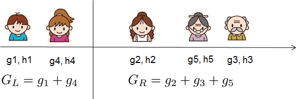
Specifically we try to split a leaf into two leaves, and the score it gains is

$$\text { Gain }=\frac{1}{2}\left[\frac{G_{L}^{2}}{H_{L}+\lambda}+\frac{G_{R}^{2}}{H_{R}+\lambda}-\frac{\left(G_{L}+G_{R}\right)^{2}}{H_{L}+H_{R}+\lambda}\right]-\gamma$$

1) the score on the new left leaf 2) the score on the new right leaf 3) The score on the original leaf 4) regularization on the additional leaf. 5) We can see an important fact here: if the gain is smaller than $\gamma$, we would do better not to add that branch.

XGBoost Features

为什么XGBoost泰勒二阶展开后效果就比较好呢？

从为什么会想到引入泰勒二阶的角度来说（可扩展性）

当目标函数是MSE时，展开是一阶项（残差）+二阶项的形式，而其它目标函数，如 logistic loss的展开式就没有这样的形式。为了能有个统一的形式，所以采用泰勒展开来得到二阶项，这样就能把MSE推导的那套直接复用到其它自定义损失函数上。

二阶信息本身就能让梯度收敛更快更准确。这一点在优化算法里的牛顿法中已经证实。可以简单认为一阶导指引梯度方向，二阶导指引梯度方向如何变化。简单来说，相对于GBDT的一阶泰勒展开，XGBoost采用二阶泰勒展开，可以更为精准的逼近真实的损失函数。

XGBoost Tree Growth

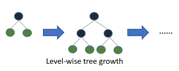
XGBoost 采用 level (depth)-wise 的增长策略，该策略遍历一次数据可以同时分裂同一层的叶子，容易进行多线程优化，也好控制模型complexity，不容易overfitting。但实际上Level-wise是一种低效的算法，因为它不加区分的对待同一层的叶子，实际上很多叶子的分裂增益较低，没必要进行搜索和分裂。 like the following image: